Introduction
In our previous article, we have seen how to get onboarded with Databricks and run your first hello world application using Spark. The first step involved creating a community edition account, creating a cluster, and running your first notebook.
Let’s pick up where we left off and build an end-to-end Spark application on Databricks. We’re using a dataset provided by the Australian government to do this. It is a CSV file that contains information about international flights to or from Australia since 2003. Spark and Databricks are often used to process and analyse large datasets that are too large for more traditional tools to handle. The dataset for this article is selected to make the tutorial quick and easy.
Fun Fact:
The volume of air traffic around the country may have a slight impact on short term weather forecast accuracy. Have a look here for more information.
There’s a handy option in the dataset page that previews the data in the CSV file. Here is a preview of the dataset.
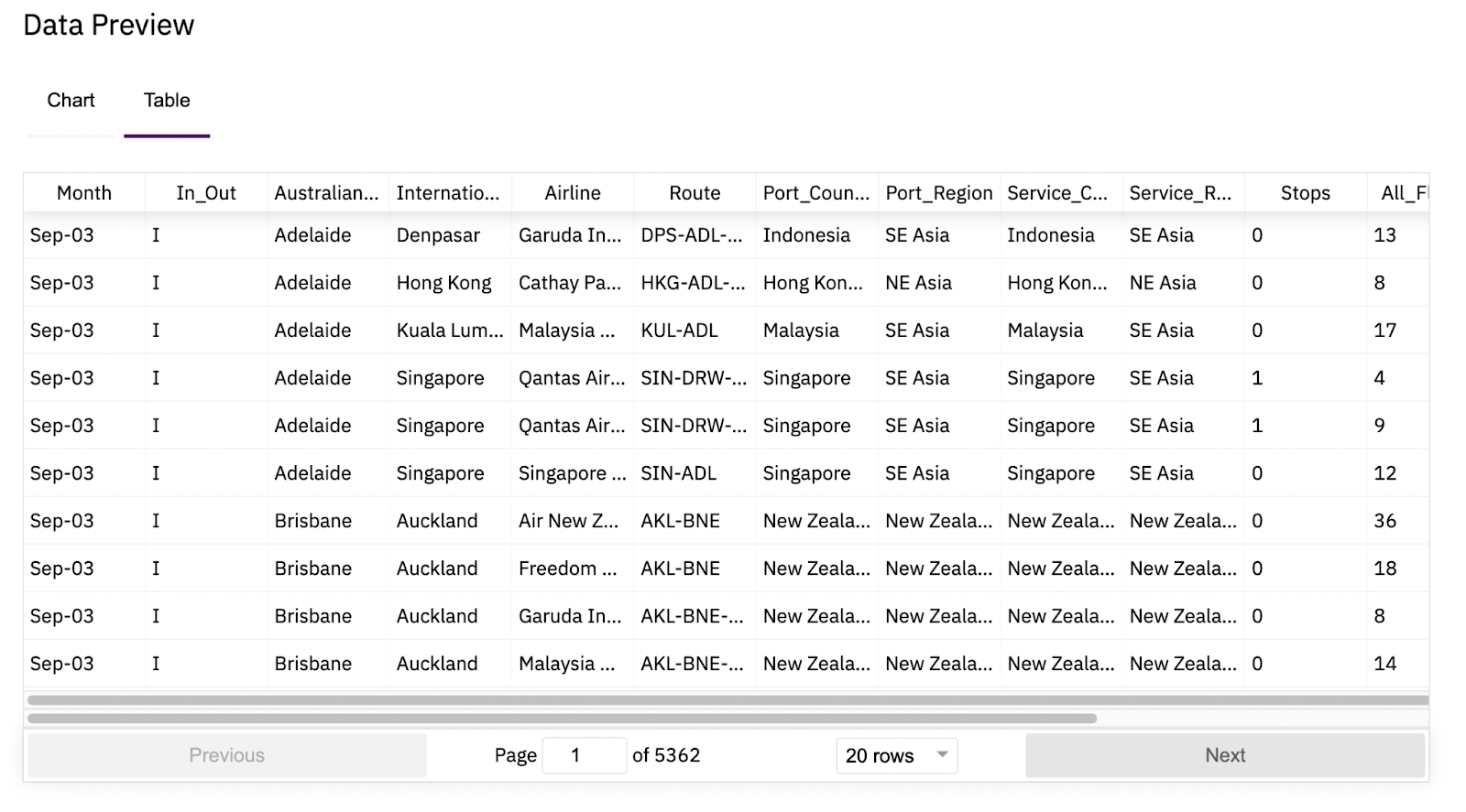
The business problem is to analyse international flights dataset for patterns or anomalies in the last 10 years or so and to investigate the impact of COVID.
Source code for this post can be found here.
Load dataset to the data lake
To load the dataset into a Databricks workspace there are a few options:
- Download the file locally then upload it manually to Databricks using the Databricks file system GUI.
- Use data ingestion tools like Azure data factory to load data from source into a destination like Databricks file system or an Azure storage account which is the preferred destination as Databricks file system (DBFS) is not recommended to host such datasets. This is not because DBFS is limited or something but because Databricks would like customers to own their data and store it independently.
- Notebooks on Databricks can run shell commands to download files to the driver node then using a Python library pre-installed by Databricks to move data to DBFS.
Option 1 is OK but it is really a manual process and it’s preferred to have something more automated and stored part of a code repository. Option 2 is for more practical use cases so we will skip it here. Option 3 is a good balance for this hello world scenario so we will stick to it.
You need first to head over to https://community.cloud.databricks.com/ and sign in to your workspace. If your cluster from part 1 is terminated, you will have to create a new cluster and wait until it is running. Unfortunately this is a limitation of community edition that terminated clusters cannot be restarted.
Follow these steps to get the dataset on Databricks file system:
- Create a fresh Python notebook connected to the running cluster.
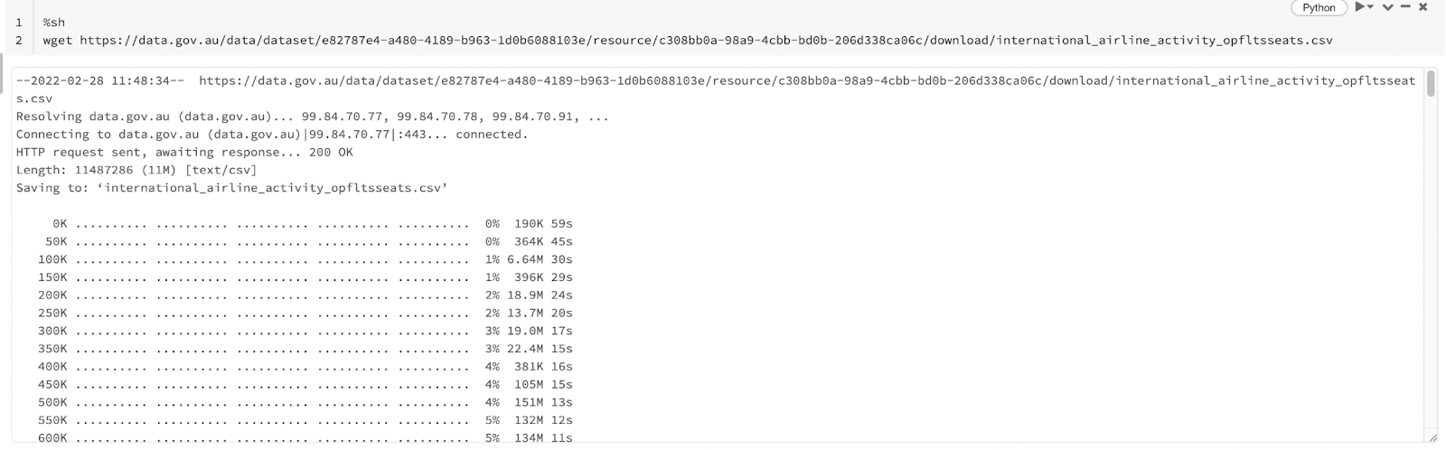
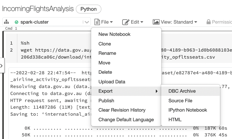
- Create a new cell to run a bash script to download the dataset. The URL can be obtained from the international flights dataset page by hovering over the download button and copying link address. The %sh at the beginning of the snippet is called a magic and it is used to run the cell using a different interpreter than the default one for the current notebook which is Python. In this case, a shell interpreter is used to run wget.
This is one of the nice features of Databricks notebooks. You can mix different languages and tools in the same notebook to make your development experience easy and fast. This does not mean it is recommended to have source code files with mixed languages but it is a common practice for experimentation and ad hoc analytics. Run the new cell and you will see the shell outcome printed showing the file is downloaded.
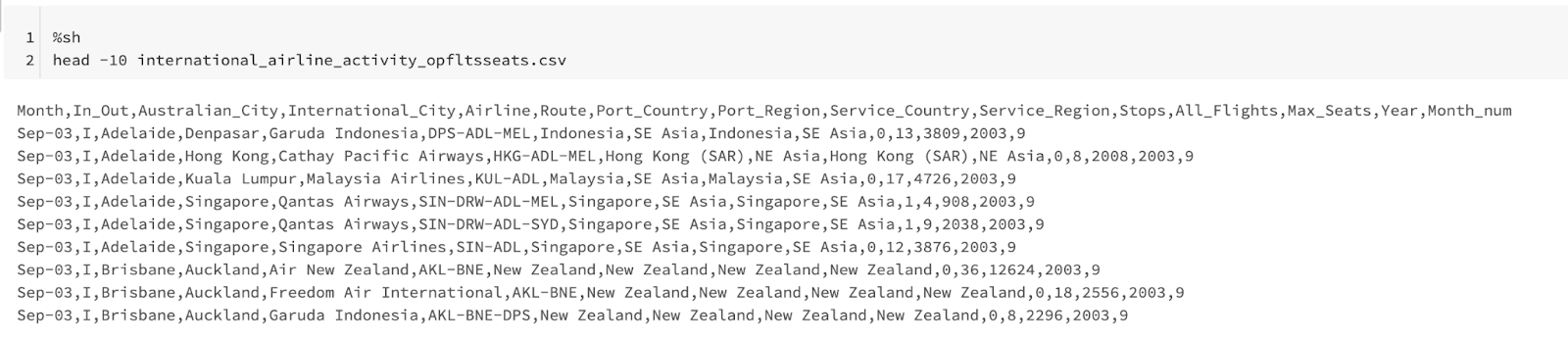
Following the same pattern, we can use another shell command to inspect file contents for a quick sanity check.
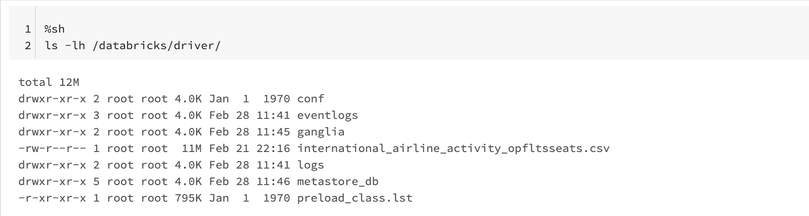
To find out what is the current working directory, an environment variable can reveal that. Another option is to just type pwd in a python cell and this will trigger an IPython magic which will produce the same effect. The current working directory in a Databricks notebook is “usually” /databricks/driver.
Then confirm that the CSV file is downloaded to the above directory.
Now we would switch back to the default interpreter which is Python and run a statement using Databricks dbutils package to move the data from the driver “local” file system to DBFS. For simplicity, consider DBFS as something like HDFS if you have used Hadoop before.
DBFS can be browsed using a GUI (after enabling an opt-in flag) or it can be directly inspected in the same notebook using the same Databricks dbutils.
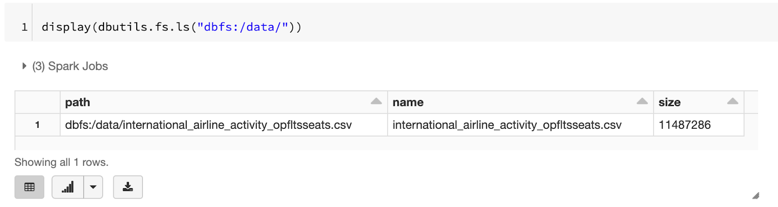
The CSV file has now been uploaded to DBFS and available for analysis.
Analyse the data
As the required data is available now on DBFS, we are ready to analyse it and find some exciting insights. If you live in Australia, the insights we will see here will not be super new to you because you are aware of the effect of COVID in the last couple of years nevertheless it is good to see how to verify known expectations using Spark.
Incoming international flights per year analysis
In the same notebook from the last exercise, create a new cell to load the data from the CSV and inspect its schema. Spark can read several file formats including the good old flat files like CSV and text files plus columnar formats like parquet and ORC used to store massive amounts of data. There are some columns that are inferred as integers and the rest are strings.
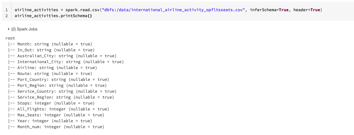
P.S. Inferring schema for CSV files is not usually a good idea but it is good enough for our case.
Now, the DataFrame loaded from the CSV file can be inspected and Databricks notebook renders it as a nice formatted table which is an improvement over the show function from Spark.

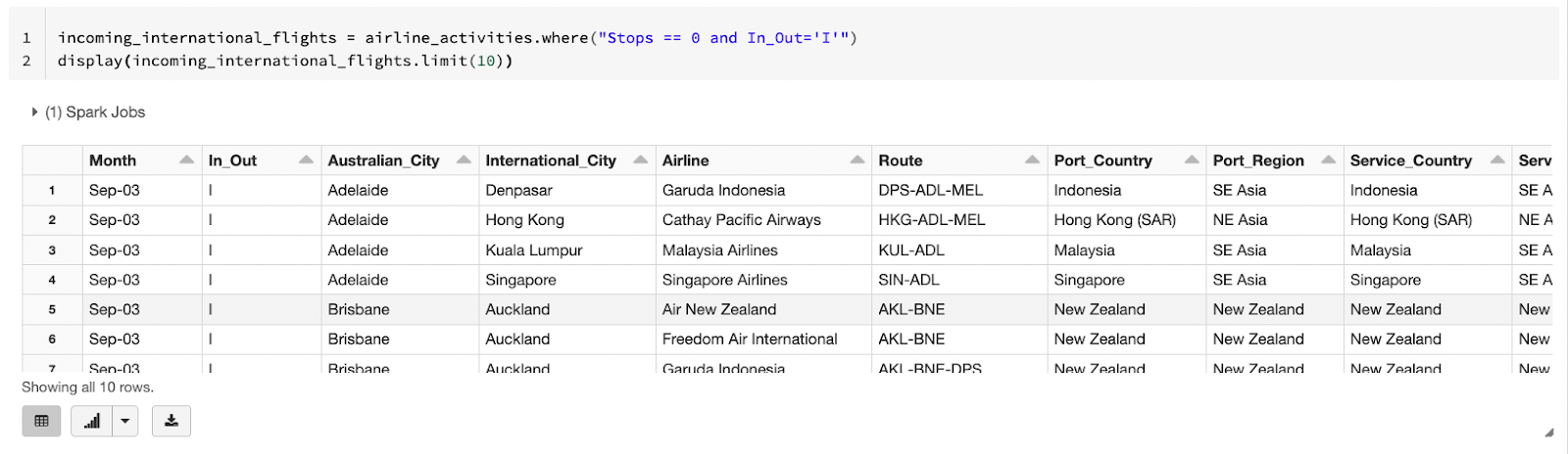
The dataset documentation file has some details on how to filter for incoming international flights only, which is to pick records where In_Out is I and Stops is 0. Spark has many ways to apply a filter on a DataFrame and one of them is to write the filter similar to a SQL where criteria. This filter will be applied because we would like to focus on incoming international air traffic only.
Let’s take the idea of using SQL skills to the next level. Spark has a SQL API that can be used to run queries on top of a certain DataFrame. But to use this feature, the DataFrame has to be registered as a table or a view first.
SQL magic (%sql) is used to write a SQL statement against the registered temporary view and analyse the number of incoming flights per year.
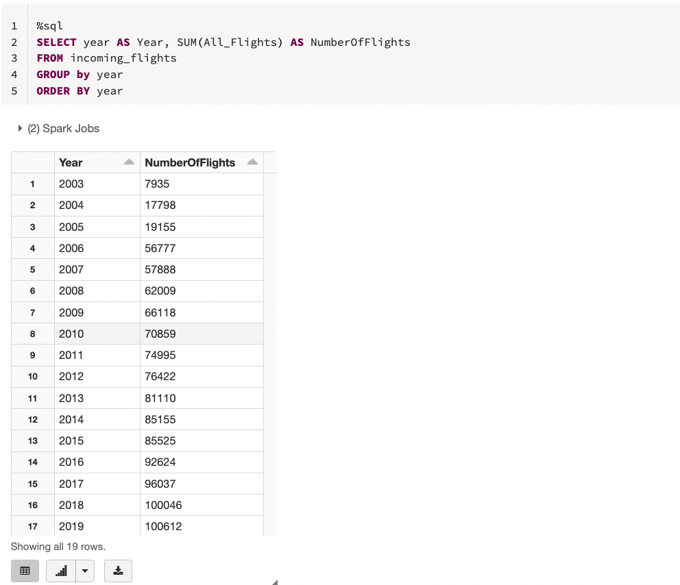
That’s quite cool to be able to run SQL queries against data sourced from a CSV file without even loading it into a relational database. You might also have noticed the small buttons below the table. It will be so hard to find out any existing facts by simply inspecting numbers so click the small arrow button beside the column chart button. It will open a small pop up to pick a chart type. Pick a line chart then use the Plot Options button to modify the x-axis to be the year and the y-axis to be the number of flights.
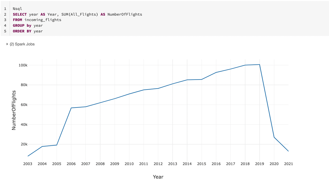
Ignoring data before 2006, it seems there was a steady growth of incoming international flights to Australia until 2019 and the rest is known. International borders were closed around March or April 2020 due to COVID. We can run similar queries to find top cities/countries with international flights to Australia pre and post COVID but let’s keep the tutorial simple.
Actually let’s not make it that simple, a GROUP BY query is not super cool. What about some window functions just to show a glimpse of what can be done.
Month over month flight count change
Let’s assume we want to analyse month over month change of number of incoming international flights. Spark SQL window functions like LAG is a tool to find the number of flights for a previous month and then the difference between the count for current month and previous month would yield the delta. Common table expressions (CTEs) make the query easy to read and write. To make the chart a bit more visible, let’s focus on years starting 2010 and switch from a line chart to a bar chart.
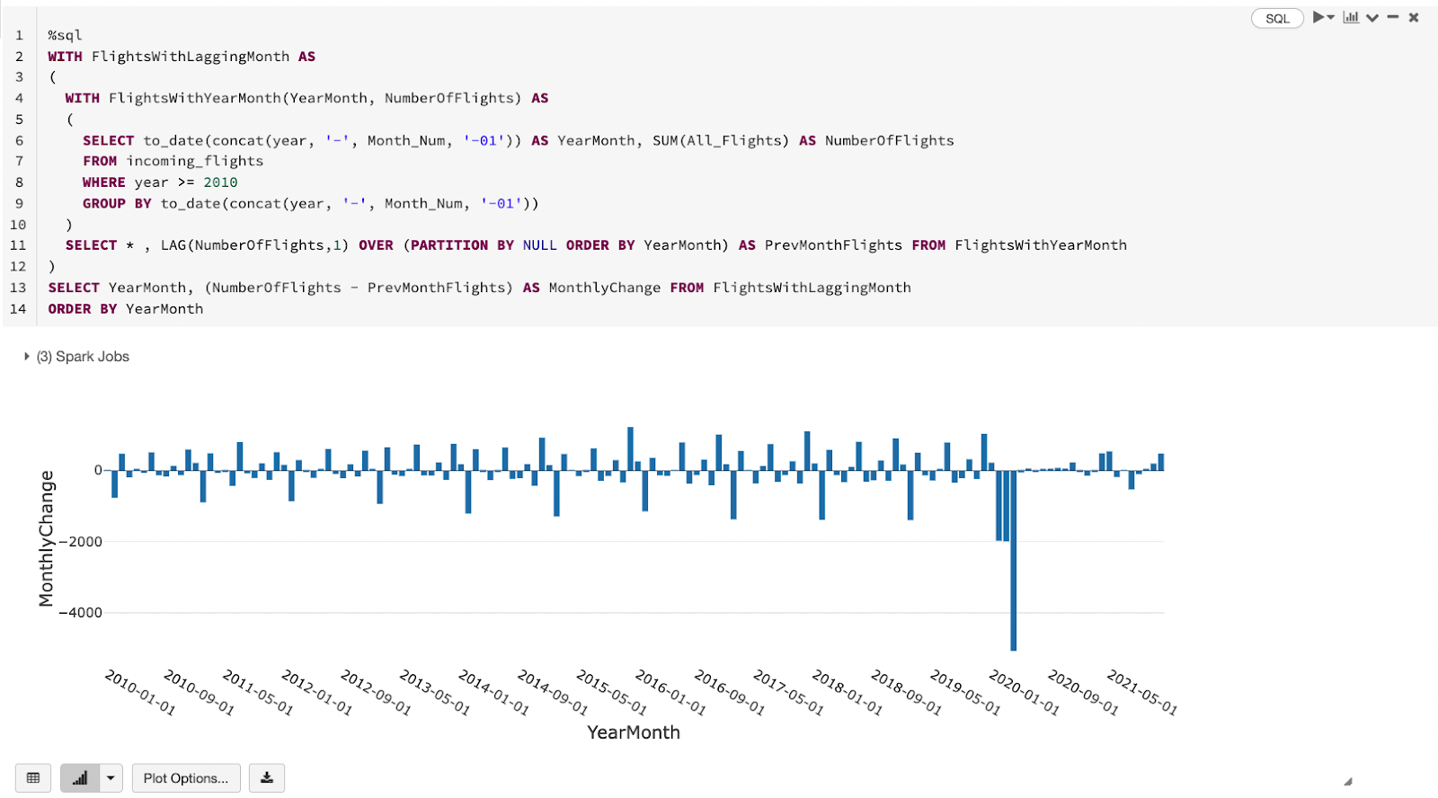
There are fluctuations as expected but the obvious patterns are:
- Before COVID, December usually had a big positive spike, could be tourism and Christmas holidays plus international students landing for the new academic year.
- Before COVID, February had a similar big spike but in the negative direction which might be the other side of the coin for December.
- February, March and April 2020 had big negative spikes due to border closure.
Now we have got a couple of queries answering certain questions about our data like number of incoming international flights per year and month-over-month change.
It wouldn’t be very optimal to always go and run the notebook manually to produce these insights. Plus we would like to export the results for other applications to consume. Let’s have a look on how to operationalise the notebook.
Warning: Databricks community edition does not have job automation feature like paid editions. So, the next steps will be done on a paid workspace. The notebook can be exported from one environment to another from the file menu at the top. You can just read on for an idea on how to operationalise the work done in the notebook.
Put stuff into production
Databricks have lots of sophisticated tools to follow best practices like CI/CD and GIT integration. But for this simple tutorial, we will only automate running the notebook we have. The notebook could run daily or weekly and be modified to export the result of the two queries into CSV files that can be consumed from other tools like Power BI or Tableau.
Modify the notebook to write results to DBFS
The same queries will be reused to produce DataFrames to write to DBFS. spark.sql API runs SQL query against registered tables or views. Repartitioning to 1 is a simple hack to produce a single CSV file because Spark as a distributed system generally produces multiple files when writing DataFrames to disk.
The second query follows the same pattern.
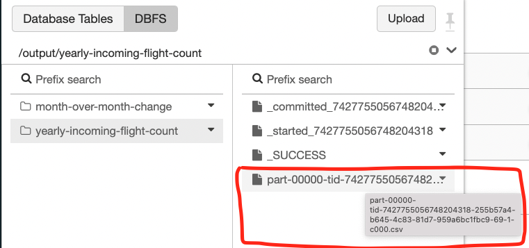
Each cell will produce a directory with a few marker files (file names starting with an underscore) plus a single CSV file.
Now give the notebook a nice name if you haven’t done it already. Just click the notebook name at the top left corner and edit the name.
Configure Databricks job
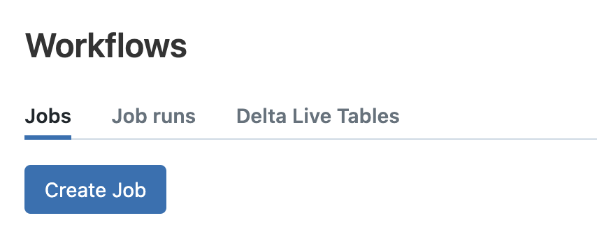
From the side menu, click the workflows button then click Create –> Job.
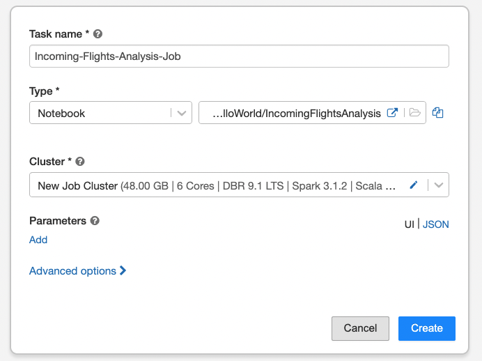
A designer for creating jobs will appear. A job can be composed of multiple tasks but in our case, it will be a single task running the notebook developed before. Fill job name then:
- Provide a task name.
- Task type should be kept as Notebook.
- Select the notebook.
- Stick to the job cluster but modify its specs to have a small number of workers/cores. It’s a single CSV file and even a single node cluster can handle it.
- Click the Create button.
A right sidebar will appear from which you can:
- Run the job on demand.
- Schedule the job to run on a timely basis.
- Set up alerts to send email notifications on success or failure.
- Change job cluster configuration, etc.
Once a triggered or scheduled job run finishes, you can inspect the status, duration and lots of extra details including notebook output itself if there is something worth investigation such as unhandled exceptions.
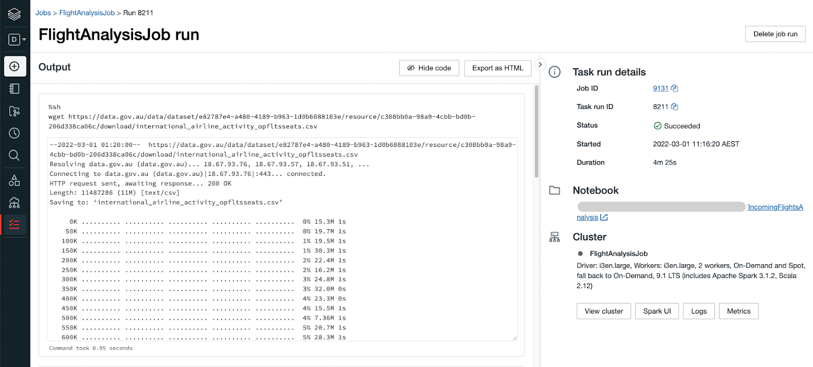
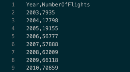
Here is the first query output data.
Wrap up
That’s was a bit more than a simple hello world example but hopefully you have some idea now on:
- Provisioning Spark environment on Databricks
- Importing data into the environment
- Performing analytics on the data
- Operationalising your work (on paid editions)
To learn more about Databricks, we have a Databricks resources page full of useful material.
Databricks provides lots of documentation and training materials on Databricks Academy. The academy has self-paced or instructor-led training courses. There are also several certification paths for tracks like data engineering and machine learning.
Here are some extra resources for further reading:
