A quick guide to forecasting in Qlik

If you’re looking to conduct some form of forecasting in Qlik, look no further!

While Qlik Sense doesn’t quite have an out-of-the-box forecasting function, in most cases a quick and easy trend line extended a few months into the future can provide most business users with the forecasting insight they need. I’ve been an avid fan of Qlik Sense across a number of projects now, and have found a few useful tips and tricks to help create a forecast using a simple linear regression method.

Here goes.

Example data source

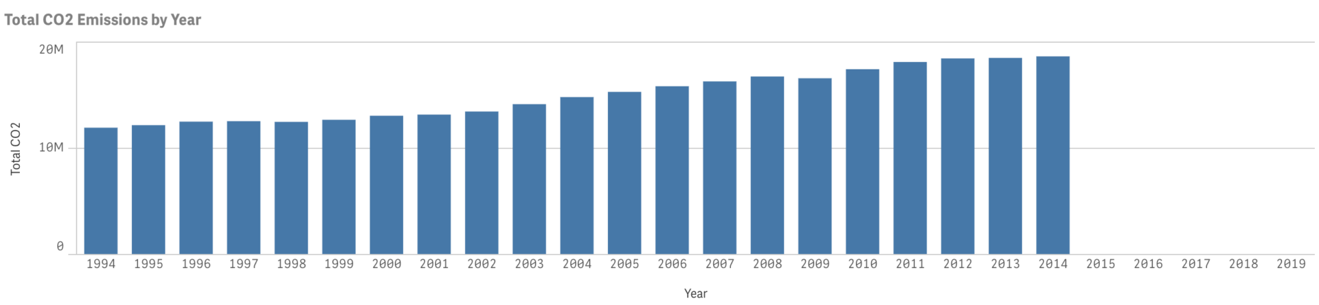
For the purposes of this exercise, I have just used the CO2 dataset available below, with annual total emissions by country from 1994 to 2014.

https://datahub.io/core/co2-fossil-by-nation#data

The question?

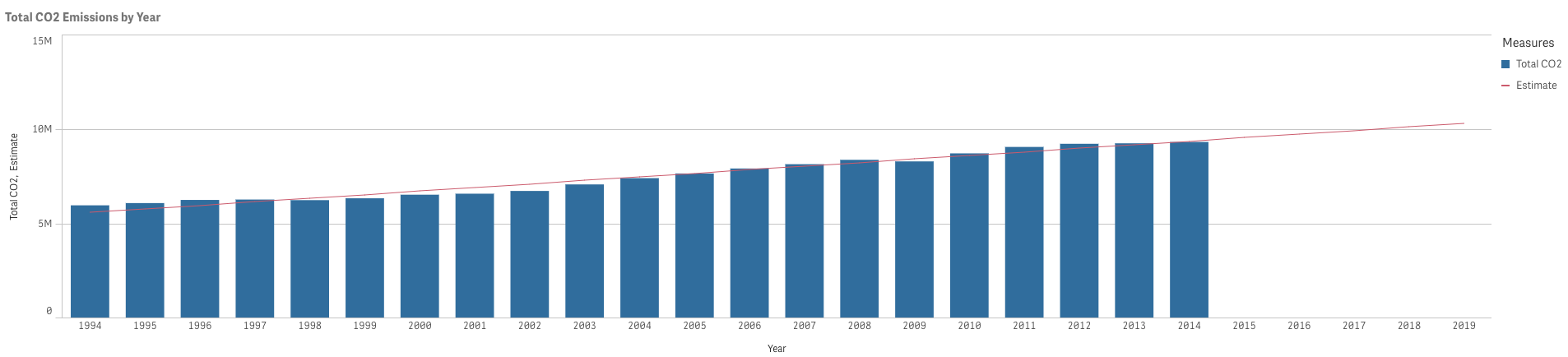
Given the total global CO2 emissions from 1994 to 2014, I want to forecast the CO2 emissions for the year 2019 by fitting simple linear regression line to the observed data.

Simple linear regression line

The equation we will replicate in Qlik Sense is Yest=b+mX, where:

• X represents the independent variable (Years)
• Y represents the variable we want to predict and explain (Total CO2 Emissions)
• M is a slope, which shows how much change in Y is caused by a unit change in X
• B is an intercept, which shows the value predicted for the Year = 0 (intercept has no meaning for time series data – more on that later)

I will not be going any further into the definitions and will cheekily leave a link to Wikipedia page for further research.

Steps

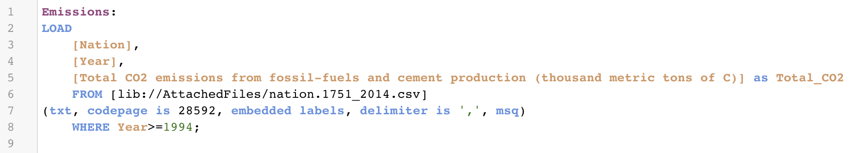
1: Load the data

My script:

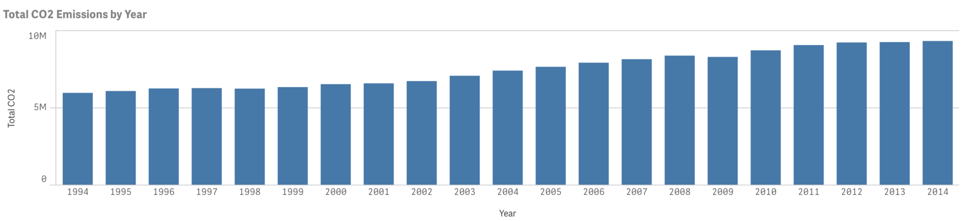
2: Plot actual values using a Combo Chart

• Year as Dimension
• SUM (Total_CO2) as Measure

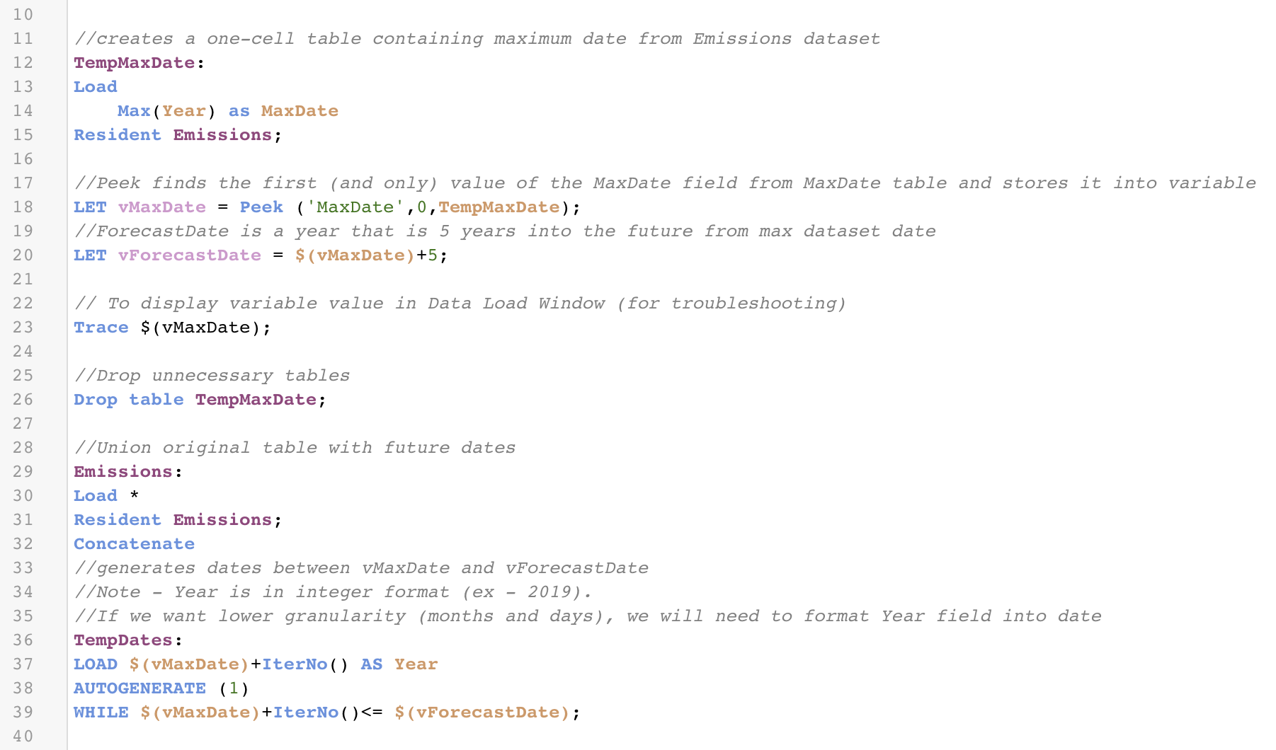
3: Extend the X-axis to include future dates

• More often than not, our dataset will include only the dates for which we have a data, therefore excluding any future dates. Linear regression without future dates plotted will result in a trend line instead of a forecast.
• To enable forecasting, we need to have future dates appended to an existing dataset.
• How do we do that?
  
  • Find max date for which we have data available
  • Find the last date in the future for which we want to have a forecast
  • Generate dates between those two
  • Union these dates with the original Emissions table (via Concatenate prefix)
• Load script with comments:

• Final result

4: Use year rank in your calculations:

• Technically, Intercept value is predicted value of Y when X=0. However, when talking about time series, predicting Total CO2 Emissions for the year of the birth of Christ just doesn’t make sense. What makes it even more confusing, is that this Intercept is 691,289,709. We didn’t have enough people to breathe that much CO2.

Why this happens is a topic for another discussion. What to do about it is a more urgent question.

• What we can do is, instead of regressing on Year, regress on Year – 1993, thus shifting X scale from absolute values (1994, 1995, etc) to relative (Year  1, 2, etc.).
• How to do it in Qlik?
  
  • We can use Script function AutoNumber(Year) to create a Year_Rank field. This function will create a unique integer value for each distinct value of the Year field.

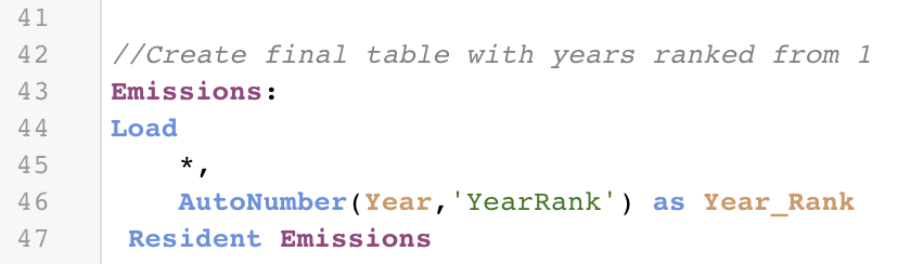
• Note! Table must be ordered by Year field (ascending order) for the ranking to work properly.
• Note! We will use Year_Rank field only for variable calculations, for the visual itself we can use Year field.

5: Calculate slope, intercept and estimated CO2 Emissions for each year

• Use LINEST chart functions:
  
  • LINEST_M will return the slope (m) of the regression defined by y = b + m*x
  • LINEST_B will return the intercept (b)
• Give values for slope and intercept
  
  • These functions will take pairs of X-values and Y-values as arguments. It’s important to remember that LINEST functions will work only if there is just one Y-value for each X-value, thus your formula for slope and intercept will depend on the shape of the data you are working with.
  • If our original table had just 2 columns – Year and Total_CO2, the criteria “one Y for each X” would be met.

• And thus our formulas would be:
  
  • LinEst_B(Total_CO2,Year_Rank)
  • LinEst_M(Total_CO2,Year_Rank)
• However, our table has 4 fields, 3 of which are dimensions:  Year, Year_Rank, Nation and Total_CO2. For a given year we can have as many Total_CO2 values, as we have nations – thus, we will need to aggregate Total_CO2 values by Year to satisfy “one Y for each X” requirement, and yet make the regression dynamically respond to our selections (ex., selecting a Nation)
  
  • Our final formulas (stored in variables vIntercept and vSlope respectively) are thus:
    
    • LinEst_B(total aggr(if(sum(Total_CO2),Sum(Total_CO2)),Year_Rank),Year_Rank)
    • LinEst_M(total aggr(if(sum(Total_CO2),Sum(Total_CO2)),Year_Rank),Year_Rank)
  • What is happening?
    
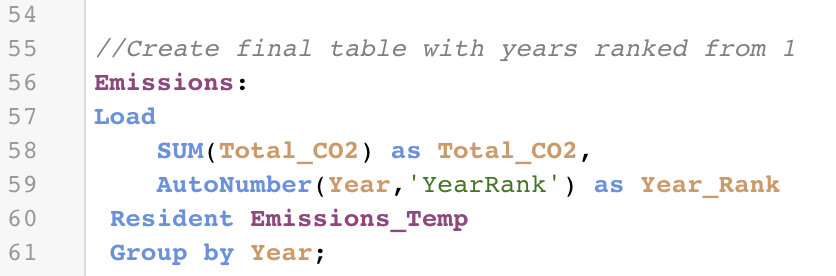
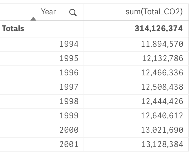
    • AGGR() function returns a temporary table with dimension values and aggregation results – “one Y for each X”:

• Then, TOTAL keyword will ensure the intercept is calculated over all possible values given current dimension selections (ie. if we select Albania nation, regression will apply the selection to our calculations of intercept and slope).
• Finally, IF function checks if the value for Total Emissions  exists. If sum(Total_CO2) is null  (which is true for years 2015- 2019), we disregard the X-Y pair from our calculations.

• Create variable vRegression:
  
  • $(vIntercept)+$(vSlope)*Year_Rank

6: Plot the estimated Total_CO2 on our combo chart:

Then the app can be downloaded!

You can download a copy of the app here.

Happy forecasting 🙂