Overview
Recently, Google announced the release of BigQuery ML, an analytics service for building machine learning models using data stored in BigQuery.
BigQuery is a serverless data warehouse designed for speed and ease of use. It can easily hold petabytes of data.
The great thing about this product is that you don’t have to export data from BigQuery to model it. You can create your model where the data is.
This post will walk you through the process of fitting, evaluating and interpreting machine learning models using BigQuery ML, using publicly available datasets.
Let’s get started.
Predicting birth weight
(Note: This example was taken from the BigQuery docs)
We’ll look at the same example as the BigQuery docs, but with a greater focus on interpretation and what you should expect to see. In addition, we’ll explain how to interpret the weights of your model, which Google hasn’t yet documented.
Step 0: Setting up
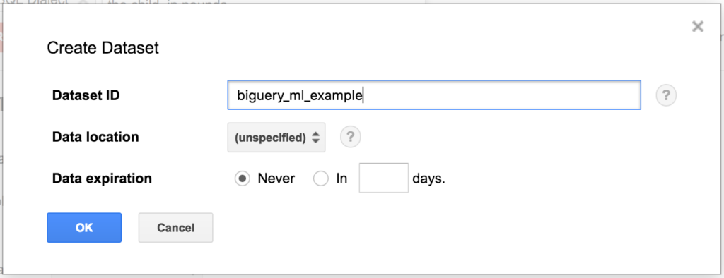
To ensure this code runs in your BigQuery account, create a new dataset called “bigquery_ml_example”.

Step 1: Understand the data
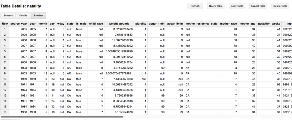
This example will use natality dataset. A table describing all registered births in the United States from 1969 to 2008. It comprises 21.9 GB of data, more than will fit in RAM in a Macbook pro.
Our goal will be to predict the birth weight of a baby. Low birth weight has been linked to a higher risk of diabetes and obesity.

A preview of the natality dataset
We will use the following columns to make our model:
- mother_age: Reported age of the mother when giving birth,
- mother_married: Whether the mother was married when she gave birth,
- mother_race: The race of the mother,
- gestation_weeks: The number of weeks of the pregnancy,
- weight_gain_pounds: How much weight the mother gained during pregnancy,
- is_male: whether the child is male.
Step 2: Create the model
We can use the CREATE MODEL function to create our model. The only options we need to specify are the model type (linear_regression) and the target variable (weight_pounds).
We want to use linear regression because we are predicting a continuous quantity (i.e birth weight.) If we instead wanted to predict a category, we would use logistic regression.
The following code will create and train our model. It should take about 15 minutes to train.
The mother_race column is a category, not a number; so we cast it to a string. BigQuery ML will automatically one hot encode category data for us. This saves a lot of effort in data wrangling.
Step 3: Evaluate the model
We can see how well our model performed by using the ML.EVALUATE function. The function takes a model name, and a table. The table should have the same schema as the table used to create the model.

The output of ML.Evaluate. There is a lot of room for improvement
From the table above average, the model will be accurate to within a pound.
Here’s how to interpret the columns:
- mean_absolute_error The average distance from the predicted value to the actual value. Lower is better.
- mean_squared_error Used for evaluating statistical significance. Lower is better.
- mean_squared_log_error Used as a numerically stable cost function by Gradient Descent for training the model. Lower is better.
- median_absolute_error A measure more robust to outliers. Lower is better.
- r2_score Coefficient of determination. Higher is better.
- explained_variance The fraction of variance explained. Higher is better.
Step 4: Interpreting the model
BigQuery standardizes numerical inputs to a regression model before it fits the model. This means we have to be very careful in interpreting the weights of the model. We can use the ML.WEIGHTS function together with the ML.FEATURE_INFO function to piece together an interpretation.
Without taking into account preprocessing, interpretation of weights is meaningless.
The following code gives us the information we need.

We can interpret the first row as saying
“All else being equal, for every 5.89 (stddev) years the mother is above 26.27 (mean) years old, we would expect to see the birth weight increase by 0.059 (weight) pounds.”
Interpreting category weights involves comparing different possible values within the category.
We would interpret the second row as saying
“All else being equal, if the mother is married we would expect to see an additional 0.224 (1.902–1.678) pounds compared to if a mother is unmarried.”
Interpreting the model weights of a regression can be challenging, but can provide useful insight.
Step 5: Prediction
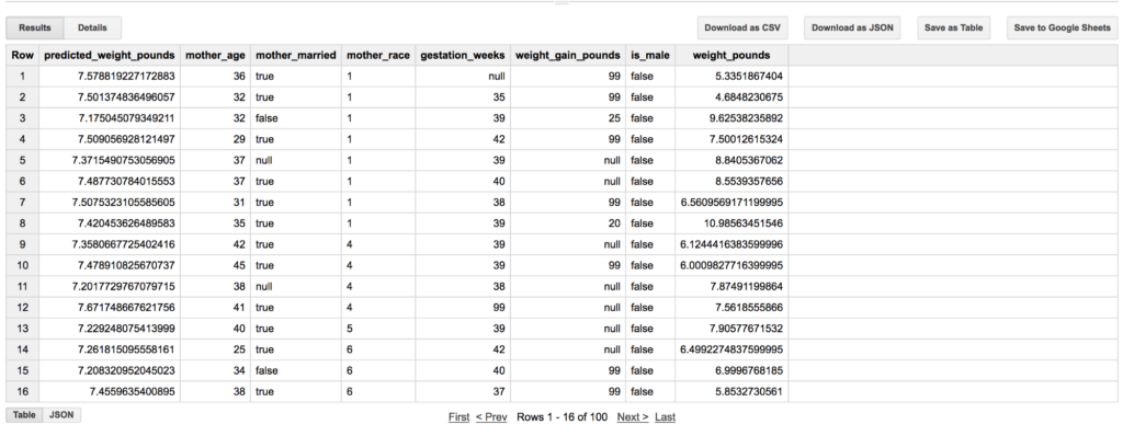
Making a prediction with the model is as easy as calling ML.PREDICT
Ensure the table you’re calling ML.PREDICT with has a compatible schema.

As the R² value indicates, the predictions generated by the model do not account for the full variation in the actual data.
You can use the prediction values as useful information in their own right, for making diagnostic plots to help you improve your model, or for imputing missing data.
Summary
You’re now familiar with how to use BigQuery ML to make Linear Regression models. We’ve gone through how to create a model, evaluate it, use the model to make predictions, and how to interpret model coefficients.
Happy Modelling!
Postscript: Using Data Science Responsibly
As Data Scientists, a way we can add a lot of value is through using our models to recommend some kind of policy. Often our interpretations of our model coefficients will lead to some sort of causal explanation, such as
“Wait longer to have a baby, since the age of the mother is linked to higher birth weight.”
This is bad reasoning and irresponsible recommendation. In fact the opposite recommendation should probably be given.
Here’s some considerations to keep in mind when extracting recommendations from your model.
Policy Considerations
Understand what policy decisions might be made as the result of your findings, and how it might be interpreted. Call out misguided interpretations explicitly.
Statistics does not give a license to be unethical. No statistical measure can justify a policy that discriminates against people based on age, class, race, religion etc.
Scientific Considerations
A model that explains little of the variation in our data is not a good basis for action. The model we made in this tutorial predicts only 5% of birth variance, so it’s really not good for making any kind of medical decision.
Correlation is not causation. Just a factor has a high weight in your model doesn’t mean it actually causes what we’re interested in. Regression analyses based on observational data should be taken as suggestive, not conclusive.